Selecting and transforming satellite bands

Introduction

In the vignette titled Grouping satellite bands by spectral and spatial resolution, vignette("satres"), the satres package is presented. It shows how to create objects of the satres class from raster files corresponding to satellite bands. It also shows how to save the data to files or export it to work with the terra package.

The main objective of this document is to show the functions available in the satres package to select and transform the satellite bands contained in satres class objects before storing or exporting them.

First, the example data and object creation functions are presented. Then, the functions that allow us to select bands are shown. Continues with other functions to transform the bands. Finally, it ends with the conclusions.

Data and object creation

In this section we discuss the data that we used in the examples, the objects of the satres class that we created and and we compare the results obtained.

Data

The data we are going to use is the same as in vignette Grouping satellite bands by spectral and spatial resolution, vignette("satres"): Two compressed files of bands from the Sentinel-2 satellite (obtained from ESA website) covering the municipality of Lanjarón in Granada (Spain) that, once unzipped, have been added with a factor of 100 (data resolution has been multiplied by 100) to be included in the package. We access the folders that contain them using the following function calls:

esa <- system.file("extdata", "esa", package = "satres")
esa_f <- system.file("extdata", "esa/f", package = "satres")
esa_g <- system.file("extdata", "esa/g", package = "satres")

We are also going to work with a vector layer of polygons with the outline of the municipality of Lanjarón, which has also been included in the package in GeoPackage format. We access the file using the following function call:

lanjaron_gpkg <- system.file("extdata", "lanjaron.gpkg", package = "satres")

Creation of objects of the `satres` class

To create an object we only need to indicate the folder that contains the satellite band files.

sr <- satres(dir = esa)

By default, only the satellite spectral bands (B01 to B12) are considered. If we want all available bands to be included, we have to indicate it using the only_spectral_bands parameter, as shown below.

sr_all <- satres(dir = esa, only_spectral_bands = FALSE)

In both cases, since all the files are contained in the same folder (regardless of how deep they are in the folder structure), the rasters that were tiles of the same work area have been merged.

In the same way, we can create independent objects with each of the folders. In this case, we are only going to consider the spectral bands.

sr_f <- satres(dir = esa_f)
sr_g <- satres(dir = esa_g)

Results obtained

We can see the results obtained so far by consulting the available spatial resolutions (it will be the same for all objects) and obtaining objects of class SpatRaster, as shown below.

sr |>
  get_spatial_resolution()
#> [1] "r1000m" "r2000m" "r6000m"

r_1000m <- sr |>
  as_SpatRaster("r1000m")

r_all_1000m <- sr_all |>
  as_SpatRaster("r1000m")

r_f_1000m <- sr_f |>
  as_SpatRaster("r1000m")

r_g_1000m <- sr_g |>
  as_SpatRaster("r1000m")

Below are the band names available for that resolution. Firstly, for the case in which we have only considered the spectral bands, then if we have considered all the bands.

names(r_1000m)
#> [1] "B02" "B03" "B04" "B08"

names(r_all_1000m)
#>  [1] "AOT"            "B02"            "B03"            "B04"           
#>  [5] "B08"            "MSK_DETFOO_B02" "MSK_DETFOO_B03" "MSK_DETFOO_B04"
#>  [9] "MSK_DETFOO_B08" "WVP"

To see the differences between the other objects, for each object, we are going to show one of the bands for that resolution.

terra::plot(r_1000m[["B02"]])


terra::plot(r_g_1000m[["B02"]])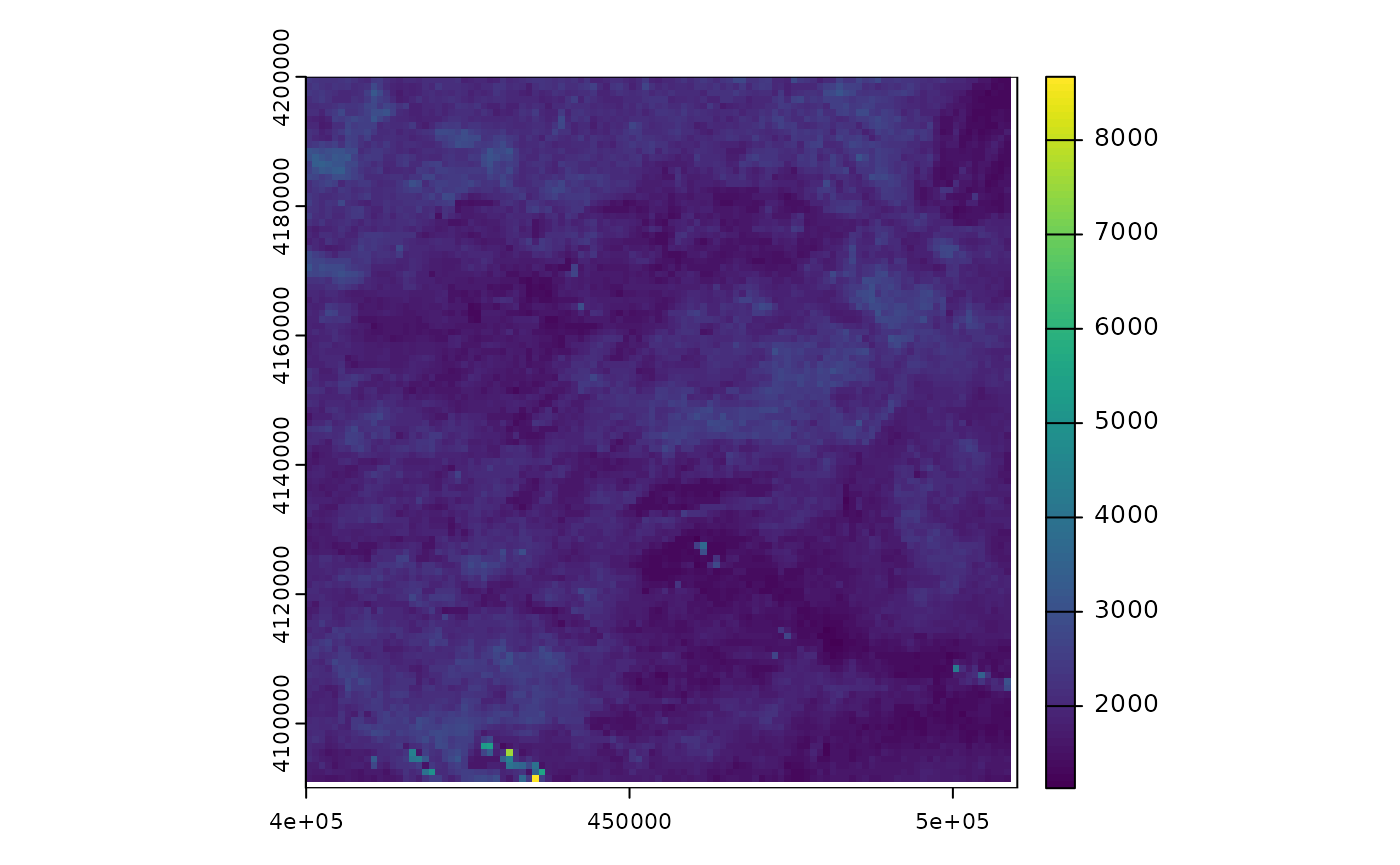


terra::plot(r_f_1000m[["B02"]])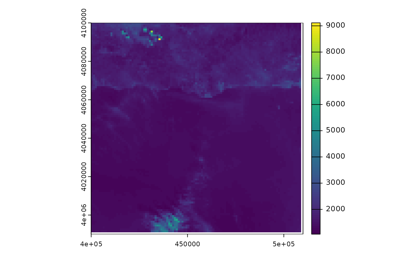

In the previous images we can see that the first raster is the result of the fusion of the two following rasters.

Band selection

First, we query the bands available for each spatial resolution; next, we select the bands and spatial resolutions we need.

Get available bands

In the previous section we have used the get_spatial_resolution() function to obtain the available spatial resolutions. We show it again below.

sr_all |>
  get_spatial_resolution()
#> [1] "r1000m" "r2000m" "r6000m"

We can consult the bands available for one or more spatial resolutions. By default they are obtained for all available resolutions, as we can see below.

sr_all |>
  get_band_names(res = "r1000m")
#>  [1] "AOT"            "B02"            "B03"            "B04"           
#>  [5] "B08"            "MSK_DETFOO_B02" "MSK_DETFOO_B03" "MSK_DETFOO_B04"
#>  [9] "MSK_DETFOO_B08" "WVP"

sr_all |>
  get_band_names()
#>  [1] "AOT"            "B01"            "B02"            "B03"           
#>  [5] "B04"            "B05"            "B06"            "B07"           
#>  [9] "B08"            "B09"            "B11"            "B12"           
#> [13] "B8A"            "MSK_CLDPRB"     "MSK_DETFOO_B01" "MSK_DETFOO_B02"
#> [17] "MSK_DETFOO_B03" "MSK_DETFOO_B04" "MSK_DETFOO_B05" "MSK_DETFOO_B06"
#> [21] "MSK_DETFOO_B07" "MSK_DETFOO_B08" "MSK_DETFOO_B09" "MSK_DETFOO_B10"
#> [25] "MSK_DETFOO_B11" "MSK_DETFOO_B12" "MSK_DETFOO_B8A" "MSK_SNWPRB"    
#> [29] "SCL"            "WVP"

Similarly, we can also limit the query to the available spectral bands, as shown below.

sr_all |>
  get_spectral_band_names(res = "r1000m")
#> [1] "B02" "B03" "B04" "B08"

sr_all |>
  get_spectral_band_names()
#>  [1] "B01" "B02" "B03" "B04" "B05" "B06" "B07" "B08" "B09" "B11" "B12" "B8A"

Select bands

Once we know the spatial resolutions and available bands, we can generate a new satres object by selecting only some of them using the select_bands() function. If any of the parameters are not indicated, by default it considers all available values, as shown in the following examples.

sr_sel1 <- sr_all |>
  select_bands(res = c("r2000m", "r6000m"),
               bands = c("B01", "B02", "B03"))
sr_sel1 |>
  get_spatial_resolution()
#> [1] "r2000m" "r6000m"
sr_sel1 |>
  get_band_names()
#> [1] "B01" "B02" "B03"

sr_sel2 <- sr_all |>
  select_bands(bands = c("B01", "B02", "B03"))
sr_sel2 |>
  get_spatial_resolution()
#> [1] "r1000m" "r2000m" "r6000m"
sr_sel2 |>
  get_band_names()
#> [1] "B01" "B02" "B03"

Other transformation functions

In addition to selecting the bands that we need to work together, we can perform other transformation operations, such as merging the bands that are tiles of the same raster, and clipping all the bands using a polygon as a template.

Merge tiles

In section “Creation of objects of the satres class”, we have obtained the data of the area of interest by merging the rasters (in variable sr) and also in separate rasters (in variables sr_f and sr_g).

We can merge the individually obtained rasters to form a new object of the satres class, as shown below.

sr2 <- sr_f |>
  merge_tiles(sr_g)

Next, we can check that the result is the same as if we had performed the fusion when creating the original object.

terra::plot(r_1000m[["B02"]])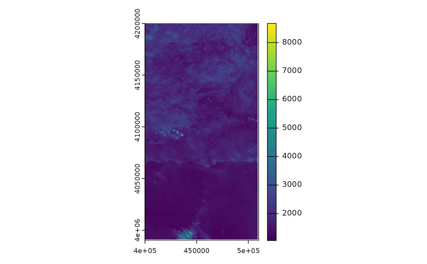


r2_1000m <- sr2 |>
  as_SpatRaster("r1000m")
terra::plot(r2_1000m[["B02"]])


sr |>
  get_spatial_resolution()
#> [1] "r1000m" "r2000m" "r6000m"
sr |>
  get_band_names()
#>  [1] "B01" "B02" "B03" "B04" "B05" "B06" "B07" "B08" "B09" "B11" "B12" "B8A"

sr2 |>
  get_spatial_resolution()
#> [1] "r1000m" "r2000m" "r6000m"
sr2 |>
  get_band_names()
#>  [1] "B01" "B02" "B03" "B04" "B05" "B06" "B07" "B08" "B09" "B11" "B12" "B8A"

Clip bands

Our objective to obtain and merge the bands is to study the area of the municipality of Lanjarón. We can clip all rasters using a polygon that represents the area of interest. In this case, we are going to use the polygon that defines the outline of this municipality.

As described in section [“Datos”][Datos], we have included a file in GeoPackage format in the package, whose name is in the lanjaron_gpkg variable. We read the GeoPackage layer we need, as shown below.

lanjaron <-
  sf::st_read(lanjaron_gpkg, layer = "lanjaron", quiet = TRUE)

To perform the clipping operation, the polygon can have any CRS, the CRS that is maintained is that of the raster layers.

sr_lanjaron <- sr |>
  clip_bands(polygon = lanjaron)

To show the result, we obtain an object of class Z and display one of the raster layers along with the vector layer used to clip them, as can be seen below.

r_lanjaron_1000m <- sr_lanjaron |>
  as_SpatRaster("r1000m")

terra::plot(r_lanjaron_1000m[["B02"]])
terra::plot(sf::st_geometry(lanjaron), add = TRUE)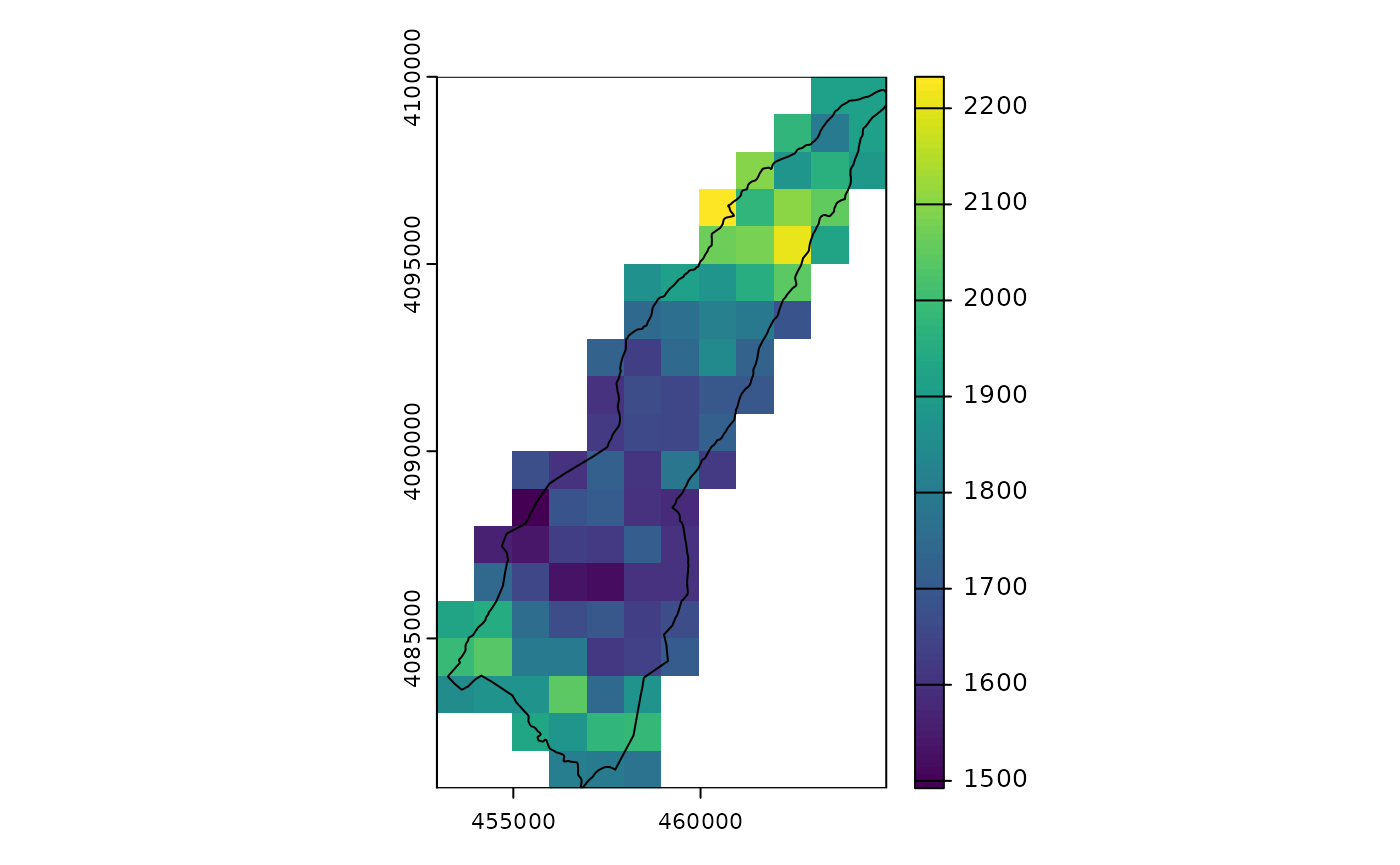

The raster layer has such a coarse granularity because of the transformation we performed to be able to store it in the package.

To show the bands available at the selected spatial resolution, we represent them graphically below.

terra::plot(r_lanjaron_1000m)

Conclusion

In this document we have shown how to query and transform the satres class objects obtained from reading raster files.

We can select a subset of the available bands and spatial resolutions, we can also merge them and clip them using a polygon.

Additionally, we can save them to files using the save_by_resolution() function, as shown in Grouping satellite bands by spectral and spatial resolution, vignette("satres").

Jose Samos (jsamos@ugr.es)

2023-10-05

Introduction

Data and object creation

Data

Creation of objects of the `satres` class

Results obtained

Band selection

Get available bands

Select bands

Other transformation functions

Merge tiles

Clip bands

Conclusion

Selecting and transforming satellite bands

Jose Samos (jsamos@ugr.es)

2023-10-05

Introduction

Data and object creation

Data

Creation of objects of the satres class

Results obtained

Band selection

Get available bands

Select bands

Other transformation functions

Merge tiles

Clip bands

Conclusion

Creation of objects of the `satres` class