Introduction
Handling geographic data efficiently involves multiple steps: transforming it to match analysis requirements, storing it in optimized spatial databases, and publishing it for sharing or integration with other systems. This package offers a comprehensive solution to streamline the transformation, storage, and publication of raster and vector geographic data.
Built upon the powerful sf and terra R
packages, this toolkit bridges the gap between local geographic data
processing and server-based geographic information platforms like
PostGIS and GeoServer. The primary aim is to simplify workflows for
users dealing with diverse geographic data needs, allowing seamless
transformation and integration of data processing, storage, and
publication in R.
In this document, the datasets included in the package, as well as other datasets used within it, are presented first. Next, a section is dedicated to each group of functions: transformation, storage, and publication; each section illustrates the functions with examples. The document concludes by summarizing the functionalities and highlighting their advantages.
Datasets
The package includes and uses the following datasets to support the workflows.
sigugr.gpkg
library(sigugr)

sigugr_gpkg <- system.file("extdata", "sigugr.gpkg", package = "sigugr")

sf::st_layers(sigugr_gpkg)
#> Driver: GPKG
#> Available layers:
#>   layer_name     geometry_type features fields              crs_name
#> 1      block           Polygon      104      1 ETRS89 / UTM zone 30N
#> 2        poi             Point      121      4 ETRS89 / UTM zone 30N
#> 3      hydro Multi Line String       11      4 ETRS89 / UTM zone 30N
#> 4 lanjaron Multi Polygon 1 4 ETRS89 / UTM zone 30Nlanjaron: A polygonal vector layer representing the boundaries of the municipality of Lanjarón, located in Granada, Spain. This data was sourced from the DERA (Datos Espaciales de Referencia de Andalucía).hydro: A multilines layer, also obtained from DERA, representing the hydrographic network for the municipality of Lanjarón.poi: A points layer representing points of interest, sourced from OpenStreetMap and clipped to the specified municipality.block: A polygon layer representing the building blocks of the considered municipality. The data was sourced from the CNIG (Centro Nacional de Información Geográfica).
sat.tif
sat_tif <- system.file("extdata", "sat.tif", package = "sigugr")

sat <- terra::rast(sat_tif)

cat(paste("-", names(sat), collapse = "\n"))
#> - B2
#> - B3
#> - B4
#> - B5
#> - B6
#> - B7
Satellite bands for the Lanjarón area, downloaded from GloVis
(USGS Global Visualization Viewer) for Landsat-8.
These bands were integrated and initially processed using the satres
package. They have been resampled to a coarser resolution to be included
in this package. These are the bands displayed as the result of the
previous code snippet.
mdt
mdt_dir <- system.file("extdata", "mdt", package = "sigugr")

cat(paste("-", list.files(mdt_dir), collapse = "\n"))
#> - MDT25-ETRS89-H30-1026-4-COB2.TIF
#> - MDT25-ETRS89-H30-1027-3-COB2.TIF
#> - MDT25-ETRS89-H30-1041-2-COB2.TIF
#> - MDT25-ETRS89-H30-1041-4-COB2.TIF
#> - MDT25-ETRS89-H30-1042-1-COB2.TIF
#> - MDT25-ETRS89-H30-1042-3-COB2.TIF
A set of Digital Terrain Model (DTM) files corresponding to the sheets of the National Topographic Map of Spain for the Lanjarón area, obtained from the CNIG. These files have also been resampled to a coarser resolution to reduce storage requirements.
clc.gpkg
clc_gpkg <- system.file("extdata", "clc.gpkg", package = "clc")

sf::st_layers(clc_gpkg)
#> Driver: GPKG
#> Available layers:
#>     layer_name geometry_type features fields              crs_name
#> 1          clc Multi Polygon      136      2 ETRS89 / UTM zone 30N
#> 2     lanjaron Multi Polygon        1      4 ETRS89 / UTM zone 30N
#> 3 layer_styles            NA        1     12                  <NA>
This GeoPackage is included in the clc
package. We will use the clc layer: a fragment of CLC data
for the Lanjarón area, stored in vector format. This layer includes the
associated style definitions, which are embedded within the same
GeoPackage (layer_styles table.). The data was sourced from
the CNIG.
Data Transformation
This module provides tools for preparing and manipulating raster and vector data to meet specific requirements. It includes the following functions, that can be grouped into two categories: clipping and other transformations.
- Clipping:
-
generate_bbox(): Creates a bounding box as ansfobject. -
clip_raster(): Clips raster layers based on polygon geometries. -
clip_layer(): Clips a vector layer using a polygon mask. -
clip_multipoligon(): Clips multipolygon vector layers with safeguards against common errors.
-
- Other transformations:
-
aggregate_rasters(): Aggregates multiple raster files within a folder. -
compose_raster(): Composes a single raster layer from multiple raster files.
-
Other transformations
We have the set of files that comprise the DTM of the area. The resolution has already been modified once, and we will change it again as shown below.
temp_dir <- tempdir()

result_files <- aggregate_rasters(mdt_dir, temp_dir, factor = 6)
The resulting files will be merged into a raster, which is also displayed below.
r_mdt <- compose_raster(temp_dir)

terra::plot(r_mdt)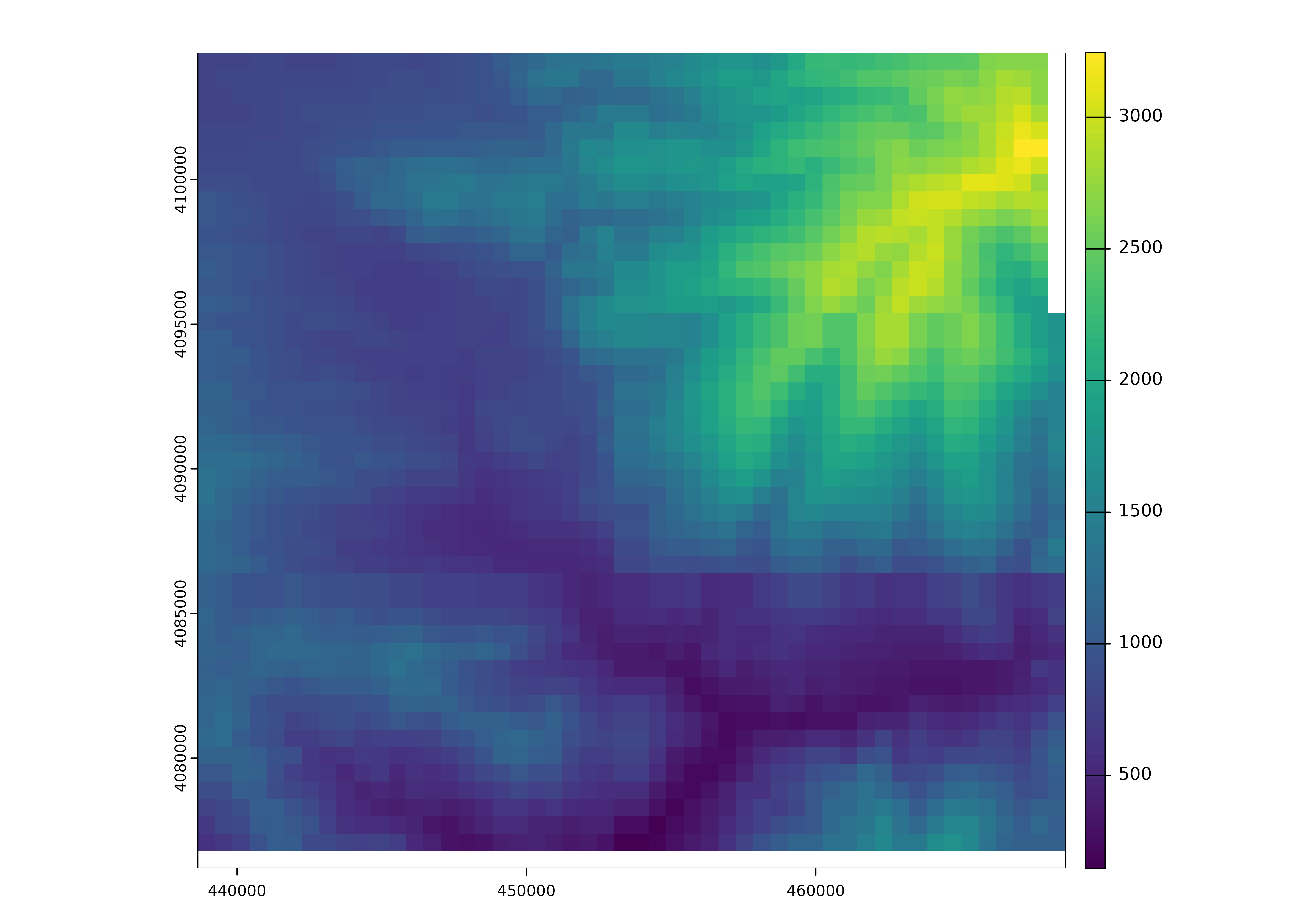
The aggregated and composed raster.
We will continue working with the DTM stored in the package, once it has been composed. When displayed in the following section, the difference in resolution compared to the previous image will be noticeable.
mdt <- compose_raster(mdt_dir)Clipping
One common operation we frequently perform is clipping various layers
using a polygon. However, in some cases, we clip them using the minimum
enclosing bounding box instead. The function
generate_bbox() can be used to obtain this bounding
box.
polygon <- sf::st_read(sigugr_gpkg, layer = "lanjaron", quiet = TRUE)

bbox <- generate_bbox(polygon)

plot(sf::st_geometry(bbox))
plot(sf::st_geometry(polygon), add = TRUE)
Polygon and bounding box.
We will crop the DTM using the bounding box and then display the result.
mdt_bbox <- clip_raster(mdt, bbox, keep_crs = FALSE)

terra::plot(mdt_bbox)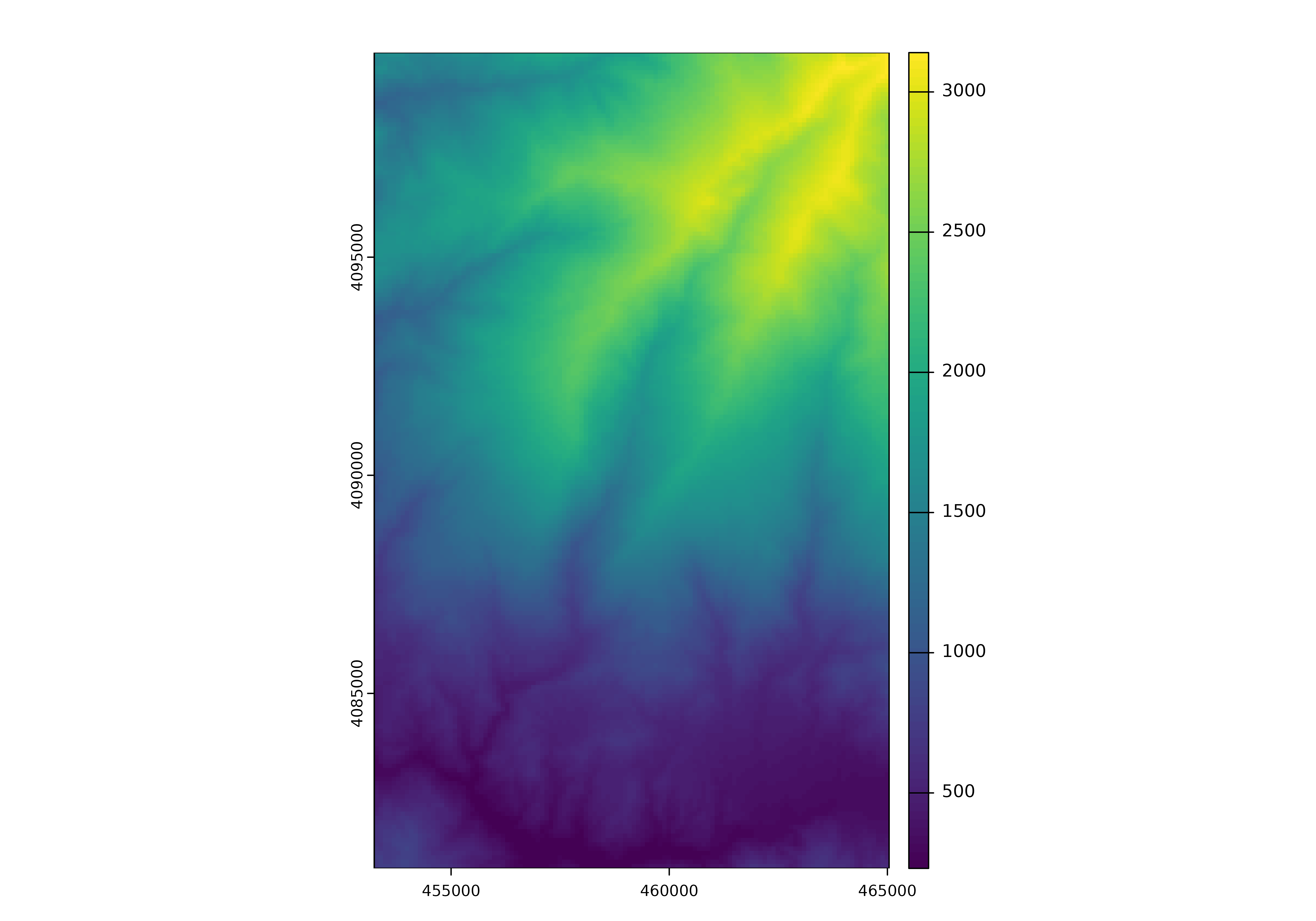
Clipped DTM.
In this case, both layers share the same CRS, but the
keep_crs parameter allows us to specify whether the
resulting raster retains the CRS of the original raster or is
reprojected to the CRS of the clipping polygon.
If it becomes necessary to change the raster’s CRS, an algorithm is applied to minimize the area being reprojected and to prevent distortions in the result.
To clip a vector layer, we will use the clc layer as
shown below. The clip_layer() function produces a layer
with the CRS of the clipping polygon.
clc <- sf::st_read(clc_gpkg, layer = "clc", quiet = TRUE)

clc_polygon <- clip_layer(clc, polygon)

plot(sf::st_geometry(clc_polygon))
Clipped CLC layer.
Clipping functions sometimes encounter issues with multipolygon
geometries; these have been addressed with the
clip_multipolygon() function, which performs the same
operation as clip_layer() but uses more computationally
expensive operations to mitigate the aforementioned issues.
To store in databases or publish the layers, they must be saved as files. Therefore, we will save the generated layers for later use.
mdt_tif <- tempfile(fileext = ".tif")
terra::writeRaster(mdt_bbox, mdt_tif, overwrite = TRUE)

clc2_gpkg <- tempfile(fileext = ".gpkg")
sf::st_write(clc_polygon, clc2_gpkg, layer = "clc_polygon", delete_dsn = TRUE, quiet = TRUE)
Data Storage in PostGIS
This module facilitates the storage of geographic data in a PostGIS database, offering optimized tools for handling both raster and vector data. The functions can be divided into two categories: layer storage and style management. The functions included are as follows:
- Layer storage:
-
store_layers(): Stores vector layers with geometries from GeoPackage orsfobjects to PostGIS. -
store_raster(): Stores raster datasets to PostGIS. -
store_bands(): Stores individual raster bands in PostGIS for advanced analysis.
-
- Style management:
-
copy_styles(): Copies styles between layers in GeoPackages and PostGIS. -
get_layer_categories(): Extracts style layer categories.
-
Important Note: The code from the examples in this section and the next was executed during the development of this document. However, it has been disabled afterward to avoid dependencies on the PostGIS database or the GeoServer, which are installed locally on my computer.
evaluate <- FALSELayer storage
Below, we store the following data into a PostGIS database:
The original satellite bands:
store_bands()stores each band in a separate table. Since the transformed bands had already been stored in the README document, a prefix is added to these.The generated DTM is stored using the
store_raster()function, which writes all bands to the same table. However, the DTM consists of a single band.All layers from the original GeoPackage and the newly generated CLC layer, using the
store_layers()function.
conn <- DBI::dbConnect(
  RPostgres::Postgres(),
  dbname = "sigugr",
  host = "localhost",
  user = "postgres",
  password = "postgres"
)

tables1 <- store_bands(sat_tif, conn, prefix = 'original_')

tables2 <- store_raster(mdt_tif, conn, table_name = 'mdt')

tables3 <- store_layers(sigugr_gpkg, conn)

tables4 <- store_layers(clc2_gpkg, conn)
Style management
The clc_polygon layer stored in the
clc2_gpkg file has been copied to the database. However,
the style of the original layer has not been transferred. We can copy
the style using the copy_styles() function, as demonstrated
below.
copy_styles(from = clc_gpkg, to = conn, database = "sigugr", to_layers = "clc_polygon")The result, including the layers available in the database and the
clc_polygon layer with its styles, can be viewed in QGIS,
as shown in the following figure.
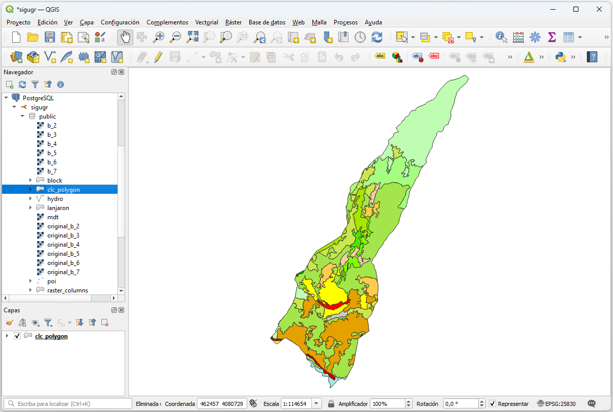
Accessing PostGIS from QGIS.
Additionally, the get_layer_categories() function can be
used to retrieve the definitions for each style code. This result can be
applied to display raster bands derived from vector layers using the
same style as the original layers.
Data Publication on GeoServer
This module focuses on publishing geographic data to GeoServer. It is
built around the geoserver class defined in the package,
with its functions implemented as methods of this class.
-
geoserver(): Manages GeoServer connection objects using an S3 class. -
register_datastore_postgis(): Registers PostGIS databases as GeoServer datastores. -
publish_layer(): Publishes vector layers to GeoServer. -
publish_layer_set(): Publishes a set of vector layers to GeoServer. -
publish_raster(): Publishes raster datasets to GeoServer. -
publish_bands(): Publishes individual raster bands as separate layers in GeoServer.
The following demonstrates how to publish all vector layers from the
database. First, the geoserver() function is used to create
an object with the connection parameters and workspace. Next, the
PostGIS database is registered as a datastore using the
register_datastore_postgis() function. Finally, vector
layers can be published individually with the
publish_layer() function or in bulk using the
publish_layer_set() function, which connects to the
database to retrieve the available vector layer names.
gso <- geoserver(
  url = "http://localhost:8080/geoserver",
  user = "admin",
  password = "geoserver",
  workspace = "sigugr"
)

gso <- gso |>
  register_datastore_postgis(
    "sigugr-db",
    db_name = 'sigugr',
    host = 'localhost',
    port = 5432,
    db_user = 'postgres',
    db_password = 'postgres',
    schema = "public"
  )

gso |>
  publish_layer_set(conn)
On the other hand, rasters stored in files can also be published, as
GeoServer does not support using PostGIS as a datastore for rasters. For
rasters, it is possible to differentiate between publishing the entire
raster with all bands together using the publish_raster()
function or publishing each band individually using
publish_bands(). In the latter case, a prefix is also added
to distinguish these bands from those already published in the README
document example.
gso |>
  publish_raster(mdt_tif, layer = 'mdt')

gso |>
  publish_bands(sat_tif, prefix = 'original_')
As with PostGIS, GeoServer can be accessed via QGIS using WMS. The following figure shows the layers available on the server within the workspace defined in the connection, along with a display of one of the layers -specifically, the DTM generated earlier in this example.
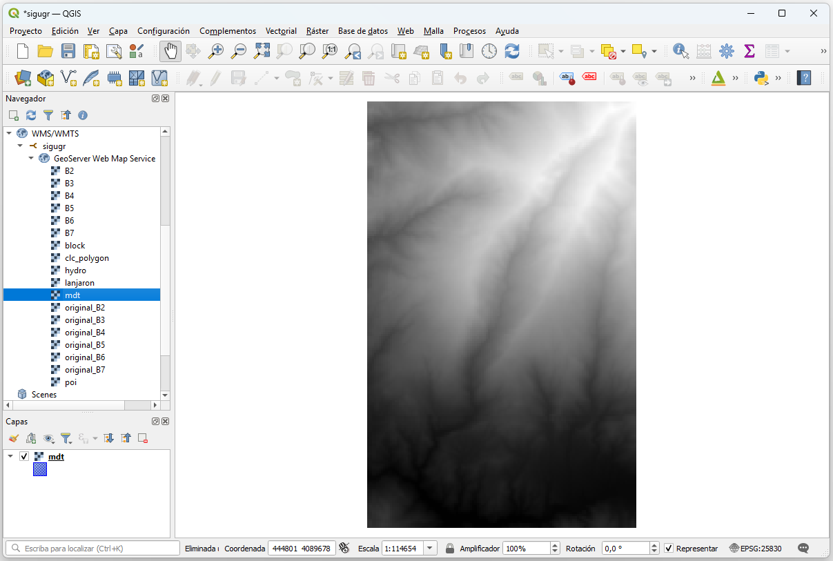
Accessing GeoServer from QGIS.
Conclusions
This package provides a framework for geographic data management, covering the lifecycle of data from processing to publication. The package enables users to:
- Seamlessly transform raster and vector datasets to suit various analytical and cartographic needs.
- Store geographic data persistently in PostGIS for efficient querying and analysis.
- Publish geographic data to GeoServer for visualization, sharing, and integration with web GIS systems.
The package is suitable for researchers, data analysts, and GIS professionals, facilitating robust workflows that bridge local data processing and server-based geospatial systems.
